Navigation Graph

Graph Architecture and Data Flows

When navigating in MapillaryJS, either by clicking on the map or on a navigation arrow in the viewer, the library gets a photo key to act upon. From the photo key we retrieve the data related to that key, like latitude, longitude and other properties, and create a node. The node is added to the graph.

With the node in the graph we have three tasks - showing the photo, the spatial arrows and the sequence arrows. These tasks are done in three different flows. These flows are shown in the diagram below. The green text indicates that a potential data request is done. Whenever the data needed is already cached, no request is made and the data is retrieved directly from the cache instead.

In the left-hand flow we retrieve the photo and the mesh used for 3D transitions. When both of these have been retrieved, the photo is shown in the viewer. This flow is independent of the other flows and their load times and therefore fast.

In the right-hand flow we retrieve the sequence data, determine the sequence edges and enable the sequence arrows accordingly.

The middle flow is a bit more involved and will be explained in more detail below. In short, we first retrieve tiles. Tiles are rectangular areas at different positions and sizes, distributed in a grid structure on the world map. We use S2 cells with a size of about 75 x 75 meters in MapillaryJS. Each tile contains photos distributed according to their GPS positions. After retrieving the tiles, spatial data for adjacent nodes is retrieved. Based on this, together with the sequence data from the right-hand flow, we compute spatial edges - the underlying data for displaying the respective spatial arrows that are shown in the viewer.

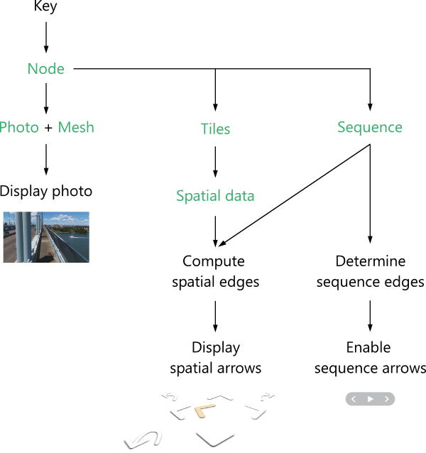
Architecture of the MapillaryJS 2.0 navigation graph

The rest of this page focuses on the flow in the middle and how we determine the spatial edges.

Determining the Spatial Edges

The spatial edges flow starts with determining which tiles are needed for a certain node. Because the node has a GPS position, we know which tile it belongs to and can act accordingly. Also, because we run Structure from Motion, we can make use of the improved computed GPS positions to make later calculations more accurate.

We retrieve tiles containing only basic node information like photo key, latitude and longitude to keep the amount of data low. For that reason we have to retrieve the spatial node data needed to determine good candidates for spatial edges at a later point in time.

We want to ensure that all the surrounding data that is needed for computing the edges in all directions is retrieved before doing any calculations. A bounding box with a side of 40 meters (dashed green square in the figure below) gives us every other node within at least 20 meters in all directions. When our node (the green dot in the figure) is in the middle of a tile (the black square) it is straightforward because all the other nodes in the bounding box will belong to the same tile and only that tile needs to be retrieved.

Our node of interest with its bounding box within a tile

When the node position is close to the boundary of the tile, a little more work is required. The bounding box will overlap multiple tiles (as seen in the next figure) and all of them need to be retrieved to ensure that all other nodes within the bounding box are available when computing the spatial edges.

A bounding box that overlaps multiple tiles

Let's continue with the multiple tile example. When all the tiles have been retrieved, the other nodes within the bounding box (represented in the figure by the yellow dots) can be determined. For those nodes the spatial data required besides the geographic coordinates is retrieved. Mind that nodes are usually not uniformly distributed in the tiles but more densely populated along roads (e.g. let's imagine that our example shows a large park).

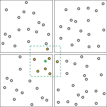
Adjacent nodes within the bounding box

Now that all the spatial data for the nodes in the bounding box has been retrieved, we can calculate the spatial edges and notify the render process to ensure that spatial arrows are shown. In this case we see four blue nodes that qualify as targets of edges from our source node. These nodes need to satisfy a number of constraints based on relative viewing direction, moving direction, and distance, among other things, to qualify as edge targets in a certain direction.

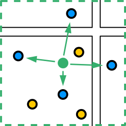
Adjacent nodes that qualify as edge targets in certain directions

Once the edges for our green source node have been determined, we also retrieve the data for the blue target nodes and determine their edges in the same way in a pre-caching algorithm to ensure that there is no or minimal loading time when navigating.

Summary

The graph architecture was implemented to decrease load times by focusing on showing the photo as fast as possible, and independently creating the navigation arrows while loading less data.